How PayLead takes full advantage of model monitoring

Model monitoring involves closely monitoring the performance of machine learning models in production to identify and address issues such as poor technical performance and inaccurate predictions. By doing so, AI teams can optimize the performance of their machine-learning models and ensure they function at their best.

Why is model monitoring necessary for any data project?

Because models perform worse in production than they do in development environments. And in too many cases, such models can become obsolete or degrade over time if their performance is not monitored. That’s why the production release of a Machine Learning model should never be the final step of any data project.

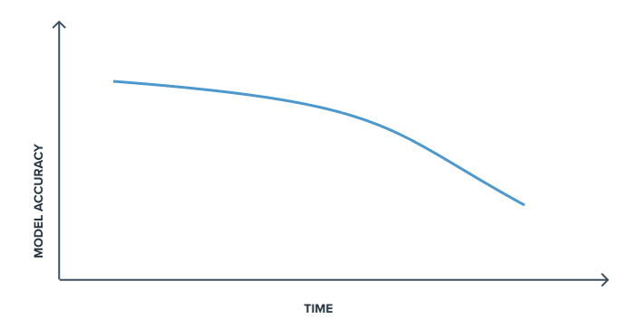
The data on which models are based is dynamic and evolves over time. These models can start to behave unexpectedly when exposed to new data, and the relations learned at time t, may no longer be accurate at time t+1.

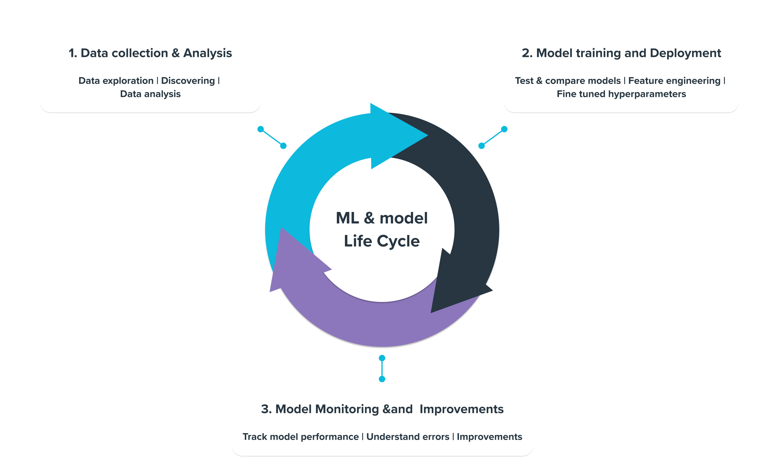
Model monitoring refers to all the techniques used to track the performance of a model in production and thus quickly detect certain drifts and potential errors in the predictions made. This is done to improve models continuously and is an essential component to be integrated into the workflow of a data project as soon as one or more models are confronted with reality.

In addition, the monitoring model guarantees transparency and confidence: It allows data stakeholders to be convinced of the performance of the model used in production while better understanding how it works and the various points of improvement. This becomes even more critical when many models are deployed, as manually monitoring all their behaviors becomes impossible.

2. Drifting main concepts

Nowadays, most Machine Learning systems are built from historical data and are therefore supposed to reflect reality as it was during training. However, as we have seen, the data and the complex relationships learned by the models evolve over time. This is known as the drift concept.

It is essential to adopt an adaptive learning strategy to monitor models implemented in production in dynamic environments based on the detection of this drift. The goal is to alert the data stakeholders of the identified drift as quickly as possible to solve the source of the problem in the most efficient way.

Let's define this concept and recall its importance in monitoring procedures.

Mathematically, the concept of drift between time t and t+1 can be defined as follows:

With P_t(X,Y) corresponding to the joint probability of the input variable X and the output variable y at time t. According to the formula of conditional probabilities, we can explain this probability as a product of 2 other probabilities: the probability of obtaining the X sample input and the likelihood of getting the output y given X.

This decomposition reflects the 2 primary sources of drift that are essential to monitoring and that we will detail below: the data drift and the model drift.

Dealing with data drift?

Data drift, the first and most obvious source of drift, refers to the phenomenon that involves changes in the data source over time.

This change can be sudden, as when a problem occurs upstream in the data pipeline of the model (like an anomaly in the data source or a preprocessing error, for example.)

This change can also be gradual if it corresponds to an underlying change in one of the statistical properties of the data distribution over time. This change usually corresponds to a slower process due to a latent change in the data source or when a new trend appears in the real world.

Moreover, each data drift has its degree of importance.

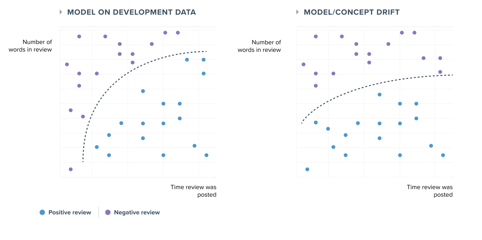
A data drift may also appear at a point in the pipeline that directly  nimpacts the decisions made by the model, as shown in the graph below:

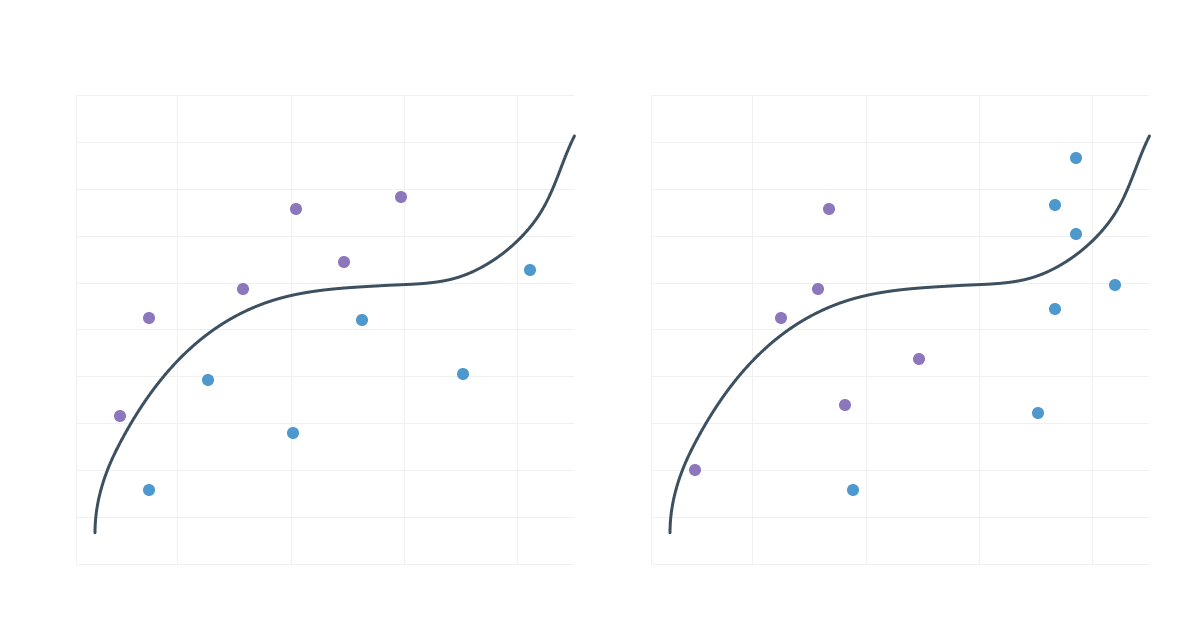
Unlike a data drift that would not directly impact the decision frontier:

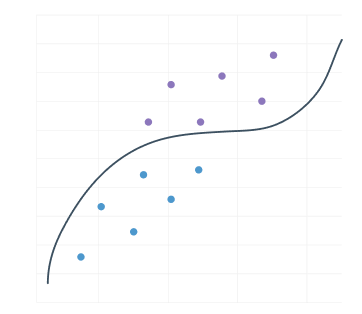
It is, therefore, essential to focus resources on identifying the data drift that causes a change in the decision boundary of a model.

Model (or concept) drift

Model drift is the second potential source of drift and refers to a change in the relationship between a model's input and output variables. Contrary to data drift, model drift will always negatively impact a model's performance since the previously learned relationships between the inputs X and the output y are no longer relevant.

It is essential to understand that this type of drift is usually gradual and can appear with or without data drift. It is triggered when certain concepts related to the real-world or business issues evolve.

What was true yesterday is not necessarily true today, and the model must reflect this change in its predictions to ensure a similar level of performance.

However, in practice, when we observe a deviation in the performance of a model, this is often due to both a data drift and a model drift, making the distinction between the two not always obvious.

PayLead business objectives

In order to guarantee the quality of the services provided by PayLead, the Data team wants to detect the drift of its models as early as possible in order to anticipate, in fine, any drop in revenue, whether for the end consumer through the cashbacks that are paid to him or for the company.

Many monitoring use cases exist at PayLead, for example :

• The monitoring of the number of transactions we received from each of our financial institution partners each day, in order to quickly detect a possible anomaly in the ingestion of transactions. However, this use case depends on many seasonal factors requiring the implementation of a forecasting model, which we will present later.
• Monitoring the types of transactions we receive. Indeed, we only reward a transaction to a consumer if it was made via a card, a deferred card or an order. We must therefore ensure that there is no drift in the type of transactions we process.
• The monitoring of the number of transactions that have matched a certain brand to detect matching anomalies. (When a new pattern is detected in the label of a transaction, or when a merchant changes its name for example.)
  

Let us now present the different methods of detecting this drift.

3. Methods to detect the drift

General concepts

Now that we understand the drift can appear at several locations in a data pipeline, we need to measure it at each point to maximize the monitoring coverage and thus gain precision in the alerts sent.

Let's take the example of a single model that, with several data sources, returns a prediction (y_pred) :

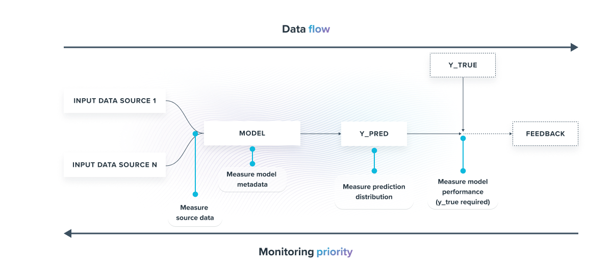
The most critical criterion to monitor is the model's accuracy because it occurs downstream in the pipeline. If an alert regarding accuracy occurs, then the other measurements must be analyzed in detail to identify the initial source(s) of the problem. In contrast, an alert upstream in the pipeline may not impact the final model's accuracy.

When a recurring accuracy measurement of a model can be tracked, it's possible to trigger an alert when it falls below a certain threshold to re-train the model or update it, as shown in the graph below

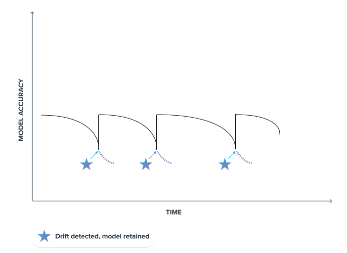
The problem with this type of supervised monitoring is that it requires simple, fast, and recurrent access to the y_true label (true output value). This requires enormous human annotation efforts.

Although moderation processes based on appropriately selected samples can be implemented, as is the case at PayLead, this technique cannot be the only one to be used in the context of a complete monitoring of a data pipeline.

There are other unsupervised drift detection techniques that monitor the distribution of data input, output, and model metadata.

Infer the drift in an unsupervised way

When several models are put into production within an organization, it isn't easy to have access to y_true for each of them. However, there are so-called unsupervised methods that allow to discover some relationships within an unlabelled data set. It is therefore with this particular method that we will address this problem and scale up the monitoring of a data pipeline.

This part focuses on the unsupervised methods that can be implemented.

Statistical test

Usually, one of the first methods is to set up statistical tests based on the observed distributions over time of the data we want to monitor.

To do this, we must define a reference period and an observation period from which we will perform these tests.

The choice of these two periods is essential and has a direct impact on the quality of the alerts sent:

• The longer these periods will be, the longer the model will take to react to a sudden drift. However, it will be more stable and more easily detect long-term trends.
• The shorter the periods, the more the model will detect sudden anomalies. It will, however, be potentially unstable and more likely to catch false alerts. If a new long-term trend emerges, it will also have difficulty detecting it.
  

fig N : Select the relevant time period for the detection and the reference part in the Data Stream

Once these two periods have been chosen, one of the first things to do is to build a monitoring dashboard by displaying the distributions over time for each period. A regular follow-up of this dashboard enables us to visually detect a significant deviation in the distribution between the two periods.

fig. N : Monitoring dashboard example for transactions type we receive for one specific financial institution

However, detecting a deviation between 2 distributions with the human eye is not always obvious and requires time, that is why statistical tests complement this visual analysis.

All that remains is to set up alerts based on a statistical test. However, the literature contains numerous tests that can be implemented within a monitoring pipeline. The choice of one of them depends mainly on the analysis studied (univariate vs. multivariate) and the nature of the fields monitored (categorical vs. continuous data).

In this article, we will focus only on two tests, one for monitoring univariate categorical variables (Z-Score) and the second for monitoring multivariate categorical variables (Population Stability Index).

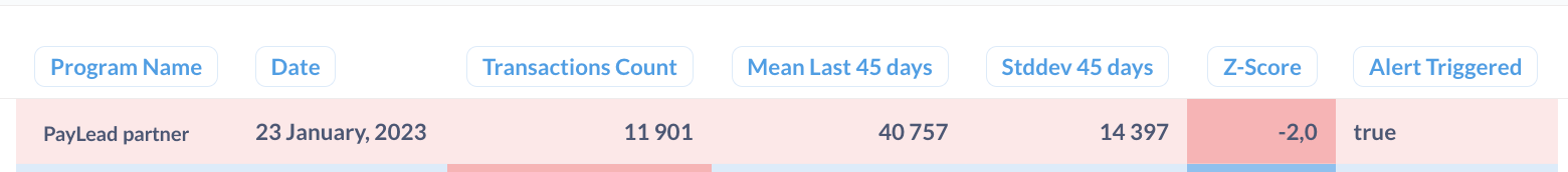
Z-Score :

Z-score is a parametric measure that takes 2 inputs as parameters: mean and standard deviation, and describes how many standard deviations away a given observation is from the mean.

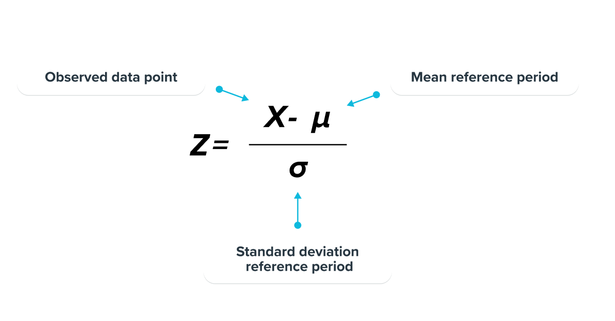
This statistical test assumes as an initial hypothesis that the observed values result from a normally distributed population.

The further the observed data point is from the mean, the more likely it is considered to be an anomaly. It then remains to define a threshold corresponding to the number of standard deviations from the mean for the model to send an alert.

Example of a PayLead alert to monitor the number of transactions received by our bank partner program with a threshold of +- 2 standard deviations.

Population Stability Index (PSI):

Unlike the Z-score, this test is particularly used for multivariate problems (depending on several variables).

It allows for the measurement of global change in the distribution of a population according to the evolution of each variable on which the initial distribution depends. This is the case in many monitoring problems.

The higher the final score, the more significant the change between the baseline and observed distribution. It is common to be alerted when the PSI score is above 0.2.

For example, this statistical test is used to monitor the types of transactions PayLead receives from its financial institution partners. (See the monitoring dashboard above). This test is particularly suitable as the transaction type problem depends on several categorical variables (card, deferred card, order, withdraw...)

By computing the Population Stability Index on the 2 distributions of fig N. presented just above, we obtain PSI = 0.02 which is well below the limit of 0.2 set to raise an alert. No drift is therefore detected on the type of transactions received for this financial institution partner.

However, these statistical tests are particularly dependent on the periods of observation chosen, especially when seasonality appears in the observed distributions. Some anomalies detected by these tests may be related more to a seasonal phenomenon than a true anomaly.

When such a situation appears, raising alerts using a forecasting model is preferable.

Forecasting

Forecasting models represent a field of Machine Learning that aims to predict a time series' evolution over time from a past sample. They are particularly relevant to be integrated into a monitoring pipeline, especially when trends are apparent in the data to be monitored.

From the past evolution of a feature to be analyzed, a forecasting model can infer the successive y_pred(s) in an unsupervised way and compare them to the y_true. When the difference between the two is too significant, an alert is raised.

Compared to the statistical tests presented, the advantage of this method is that it is possible to incorporate the general and/or seasonal trends in the y_true to focus only on the anomaly part, i.e., the part that interests us in the context of monitoring.

The critical concept to understand when setting up a forecasting model on a time series is Stationary.

A stationary time series is one whose statistical properties do not depend on the time the series is observed.

Obviously, a time series with well-defined trends and seasonality is not stationary. Therefore, some upstream transformations are needed to infer the y_pred.

One of the most commonly used methods when facing such a problem is to decompose the non-stationary time series into a sum of several series, each having its own characteristic, such as:

Non-stationary time series = Trend + Seasonality + Noise

Let's take one of the examples mentioned above, the number of daily transactions sent by one of our financial institution partners. As previously mentioned, the daily number of transactions received depends on several seasonal factors (in particular, there are many transactions sent at the beginning of the week which correspond to weekend transactions, as well as many transactions at the beginning of the month).

If we break down the initial time series and decompose it into several subseries, we obtain:

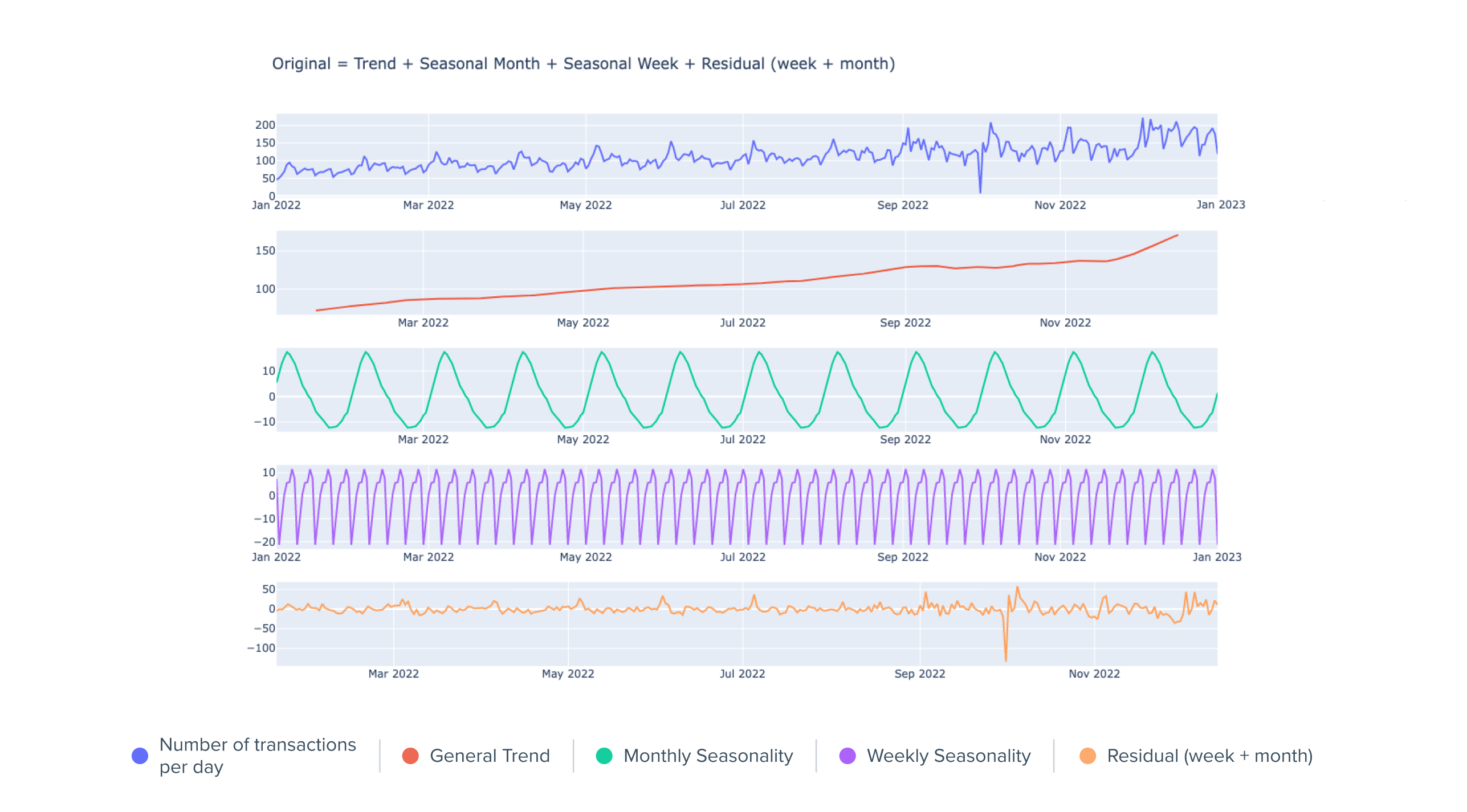
Normalized daily number of transactions sent by one financial institution partner with decomposition

Within the first time series presented on the graph above, we clearly observe 3 main trends:

• A general increasing trend: the number of transactions sent is increasing.
• A monthly seasonality: There are many transactions at the beginning of the month and less at the end. (Due to higher purchasing power at the beginning of the month)
• A weekly seasonality: There are many transactions at the beginning and few at the end of the week. (The weekend's transactions arrive at the beginning of the following week)

The first three time series resulting from the decomposition are clearly non-stationary, but their evolution is quite obvious to predict.

The last time series corresponds to the residuals, i.e. the variations of the initial time series which do not correspond to any of the 3 trends developed above. These residuals are close to a stationary time series (mean and variance close to 0 through time).

Several approaches are then possible: setting up a forecasting model on the time series of the residuals and re-composing the initial time series with the forecasts or calculating a z-score on the residual values, as these follow a normal distribution centered around 0.

Whatever one of these two methods is chosen, it is more accurate than a simple statistical test on the number of transactions received between a detection and a reference period, considering that there is a strong seasonal effect as explained above.

That is why forecasting models are so important at PayLead!

PayLead Data Stack for monitoring

Now that we have presented the main monitoring methods, here is the architecture we have implemented at PayLead to scale up and be alerted in real-time when an anomaly occurs:

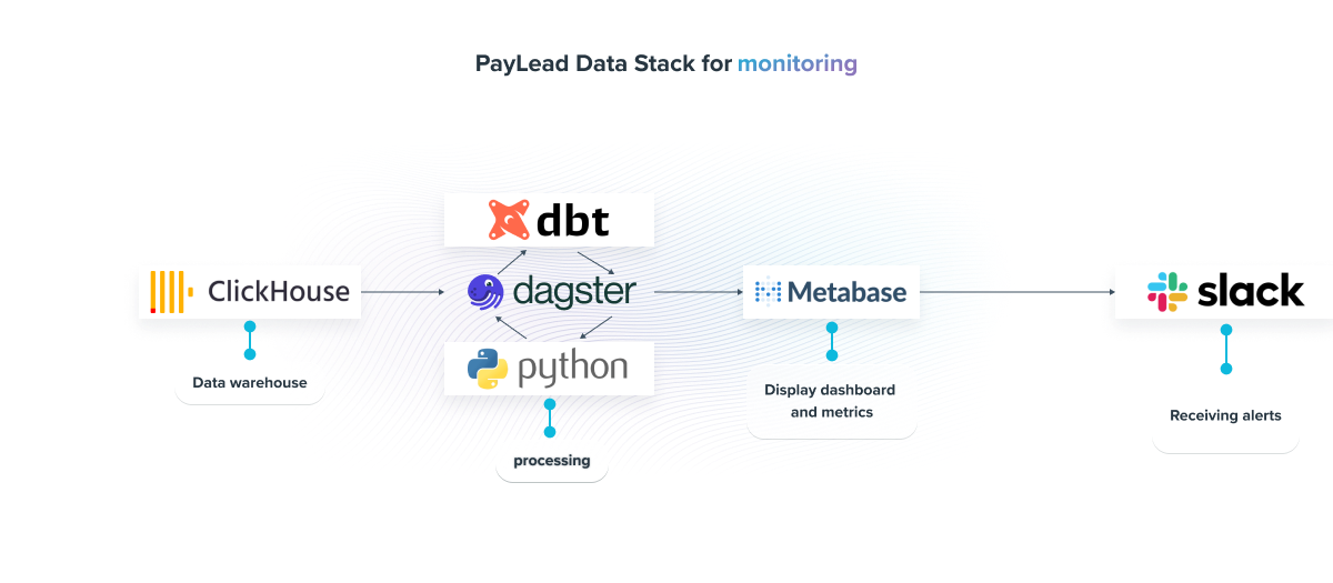
• Data Warehouse: ClickHouse, a highly scalable open-source DBMS, designed for online analytical processing, allows us to store, query, and process millions of data around the banking transaction.
• Processing: Monitoring models are nowadays mainly structured using dbt models. More complex models, such as those for forecasting, are managed via Python, offering a more developed range of tools. Orchestration is managed by dagster, which allows, among other things, to recompute the dbt marts daily and thus achieve an efficient monitoring routine.
• Display: Once the models are built, the results are displayed in Metabase dashboards, a Business Intelligence tool that gives us a permanent overview of the viability of our Data pipeline.
• Alerts: Finally, with Slack, we receive, in an appropriate channel, the warnings raised by our monitoring models.